Understanding the Entropy of a Markov Chain

Written by CasualPhysicsEnjoyer

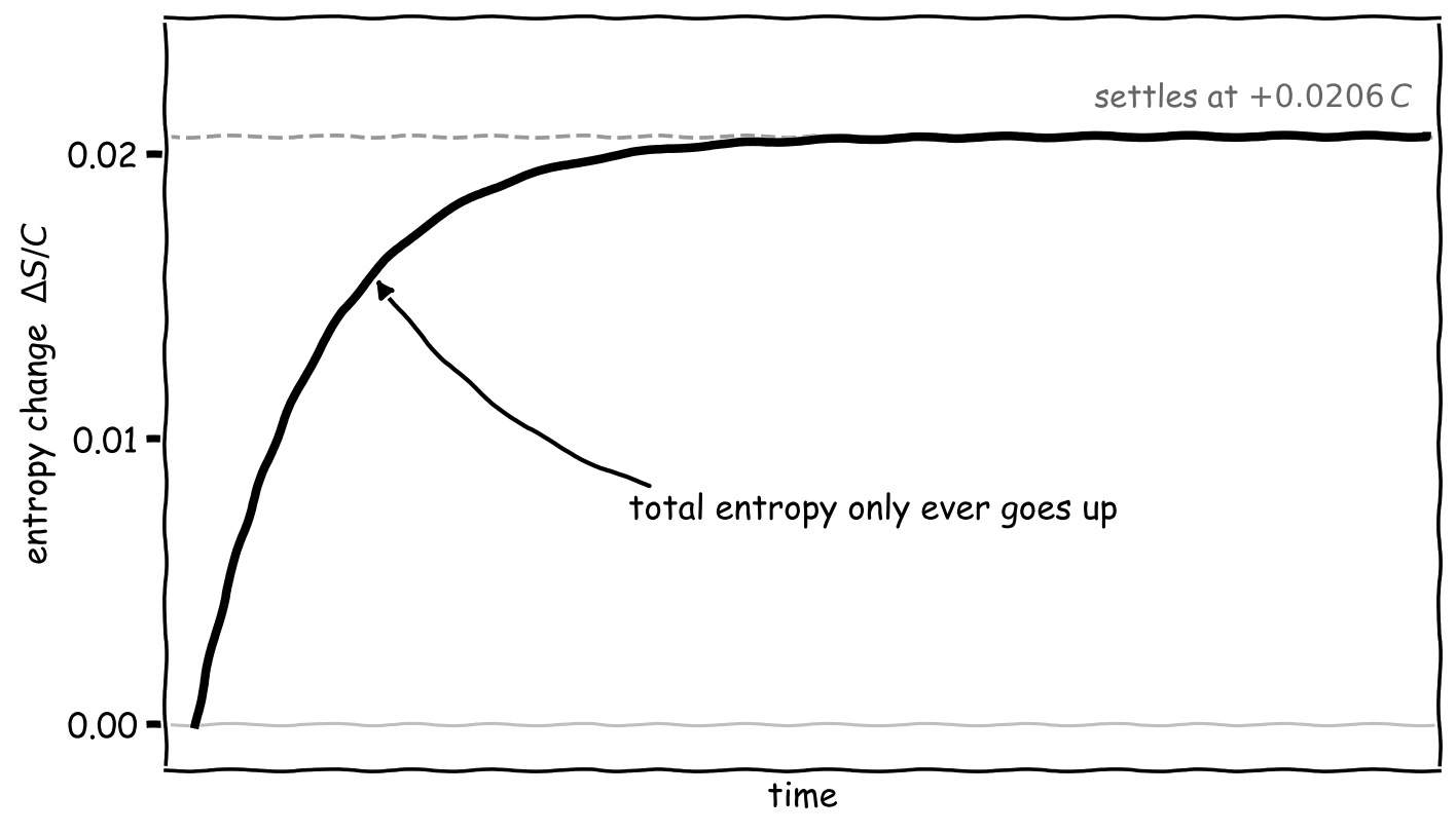
In 1865, Clausius introduced a fundamental physical quantity known as entropy. By analyzing physical processes as a series of interconnected engines, he demonstrated a core law of nature: in any irreversible process, entropy always climbs.

The Nature of Entropy

Depending on the type of process, entropy behaves differently:

Process Type	Entropy Change ( $\Delta S$ )	Example
Reversible	$\Delta S = 0$	Carnot's ideal engine
Irreversible	$\Delta S > 0$	Most natural processes

It is important to note that entropy cannot decrease spontaneously ~~unless the system is isolated~~ unless external energy is applied to the system. While you cannot measure entropy directly with a ruler or a thermometer, it remains an indispensable concept because we can derive measurable quantities from it.

"Life as entropy."

I have previously touched upon this notion, which was heavily influenced by Schrödinger (1944) and his introduction of negentropy. The premise is that living organisms maintain their internal order by consuming energy from their environment, thereby reducing their own local disorder.

However, the precise mechanics of this are often elusive. To gain clarity, I believe in using toy models—mathematically consistent simulations that allow us to observe how entropy evolves over time.

From Thermodynamics to Markov Chains

One particularly useful model is Dyson's toy model of a cell. In this framework, a cell is represented as a Markov chain that eventually settles into one of three equilibrium states, with "life" and "death" being two of the primary outcomes.

If we want to apply the "life as entropy" philosophy here, we need a definition of entropy that fits a Markov chain. This is tricky because Clausius defined entropy based on heat and temperature:

$\mathrm{d}S = \frac{\delta Q_{\text{rev}}}{T}$

How do we bridge the gap between thermal energy and a probabilistic state machine?

The Boltzmann Perspective

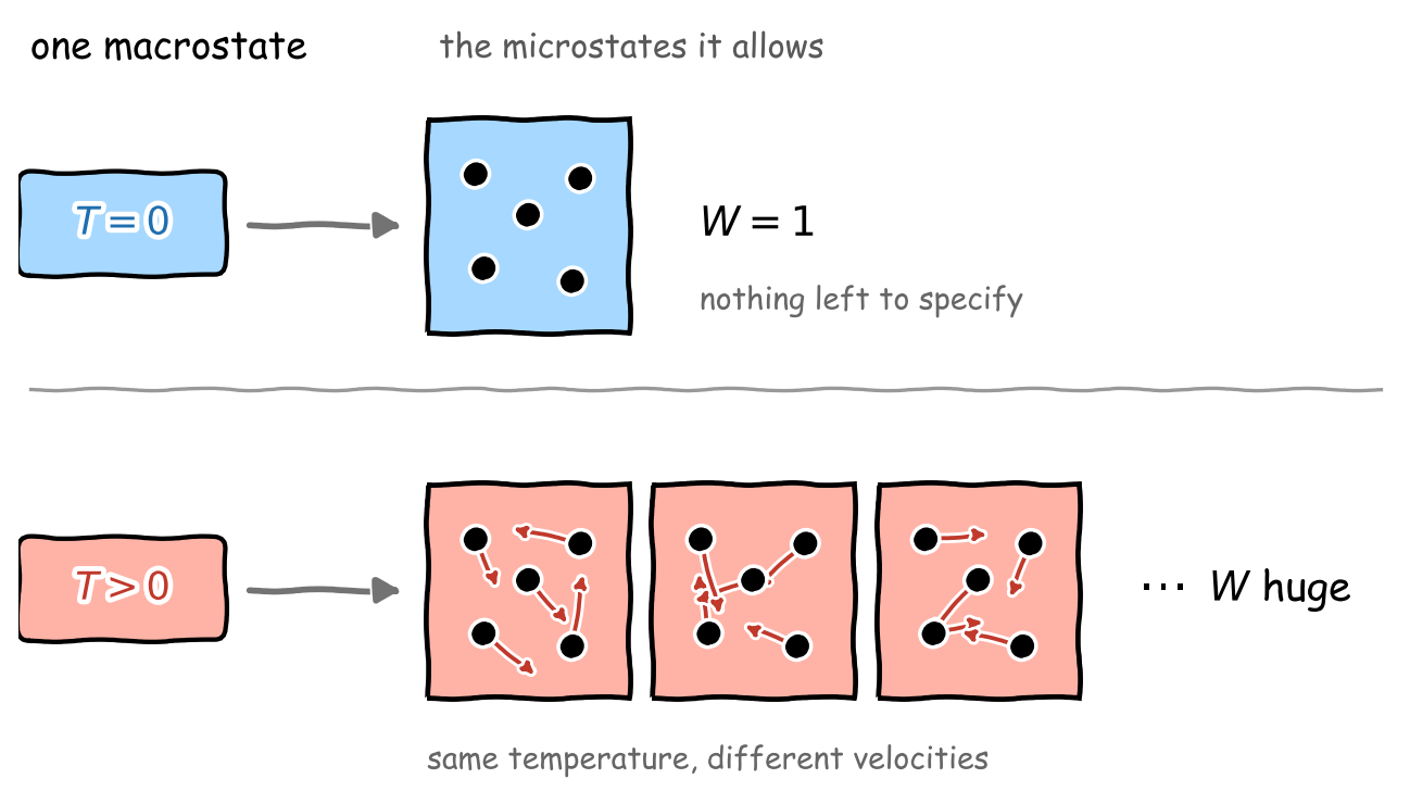
The answer lies in the work of Ludwig Boltzmann, who linked entropy to the number of possible microstates compatible with a macrostate.

Imagine observing a system's macro-variables (e.g., pressure, volume, temperature). There are countless internal configurations (microstates) that could produce those same macro-readings.

Low Entropy: A gas at absolute zero. Particles are fixed and motionless; there are very few ways to arrange them to achieve this state.
High Entropy: A hot gas. There are vast numbers of position and velocity combinations that result in the same temperature.

Boltzmann formalized this with his famous equation:

$S = k_B \ln W, \qquad W = \#\{\text{microstates consistent with the macrostate}\}$

Where $k_B$ is the Boltzmann constant. While the formula is elegant, the proof—which involves taking limits of particles with finite velocities—is complex and continues to be a subject of mathematical rigor.

A Concrete Example: Electron Spin

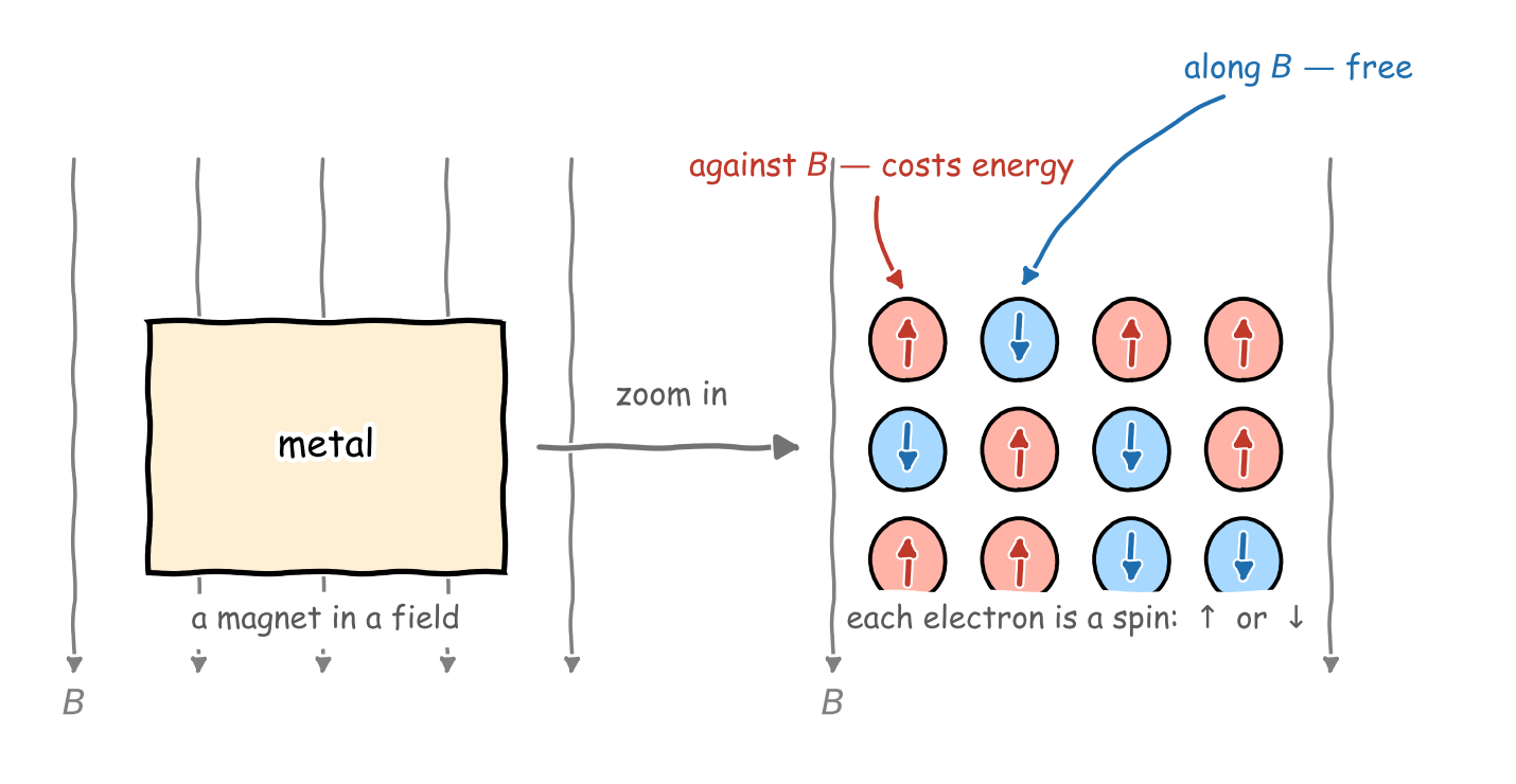
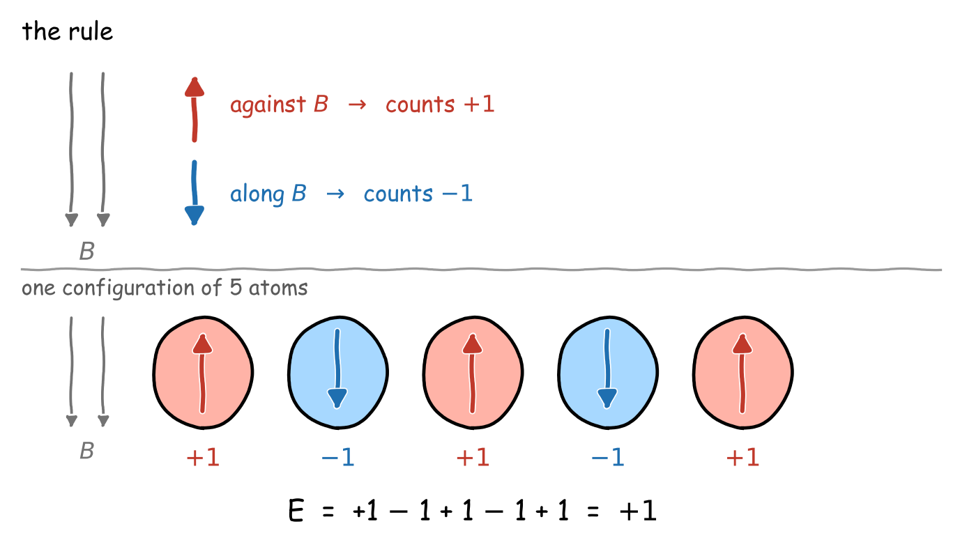
To see this in action, let's calculate the entropy of a tiny system consisting of 5 electrons. Each electron can be either spin up ( $\uparrow$ ) or spin down ( $\downarrow$ ).

In magnetic models, energy $E$ is determined by the alignment of spins: $E = n_\uparrow - n_\downarrow$

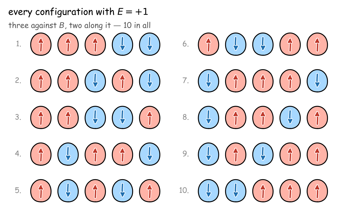
Goal: Find the entropy for a macrostate where $E = 1$ .

Step 1: Determine the number of spins. Given $n_\uparrow + n_\downarrow = 5$ and $n_\uparrow - n_\downarrow = 1$ , we solve to find $n_\uparrow = 3$ and $n_\downarrow = 2$ .
Step 2: Calculate the number of microstates ( $W$ ). We use the binomial coefficient to find how many ways 3 up-spins can be arranged in 5 slots:

import math
W = math.comb(5, 3) 
# Result: 10

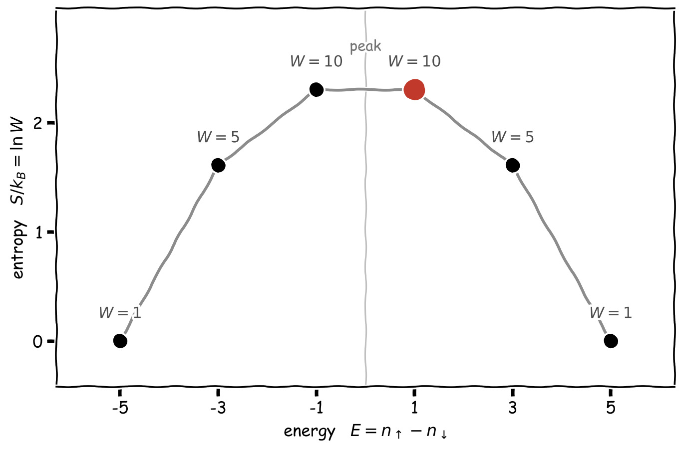
$\text{Calculation: } W = \binom{5}{3} = \frac{5!}{3!\,2!} = 10$

Step 3: Compute Entropy. Using Boltzmann's formula: $S = k_B \ln 10 \approx 2.3026\,k_B$ Alternatively, in bits: $\log_2 10 \approx 3.32 \text{ bits}$ .

By repeating this for different energy levels, we can plot entropy as a function of energy.

Applying this to Dyson's Model

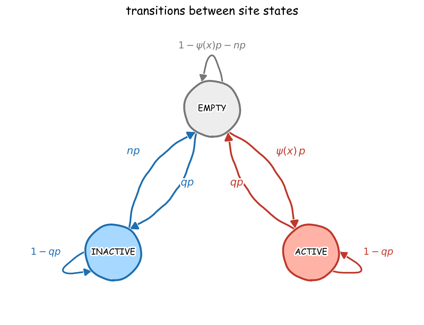
Now we can transition back to the Markov chain. In Dyson's model, we have $N$ sites, each capable of being in one of three states:

Empty
Active
Inactive

By applying the logic of counting microstates to these $N$ sites, we can determine the entropy of the system as it converges toward equilibrium.