Discrete Fourier Transform by Hand
Discrete Fourier Transform by Hand ✍️
By Prof. Tom Yeh | June 24, 2024
In the realm of signal processing, the Discrete Fourier Transform (DFT) stands as arguably the most critical methodology.
Many students find the underlying mathematics daunting. It typically involves a summation of complex terms: Where:
- is the Euler number
- is the imaginary unit
- represents angular frequency
- represents time
However, I created this exercise to prove that the math is impossibly complex it is actually just a sequence of matrix multiplications that can be performed manually.
Insight: Once you realize DFT is just matrix multiplication, it becomes clear why deep neural networks—which are also series of matrix multiplications separated by activation functions—are so adept at learning to process and analyze signals.
While a U-Net learns its specific filters from data to handle signals in the spatial domain, the DFT is the classical counterpart: a fixed transform designed by humans to analyze signals in the frequency domain as a combination of cosine waves.
🛠️ The Setup
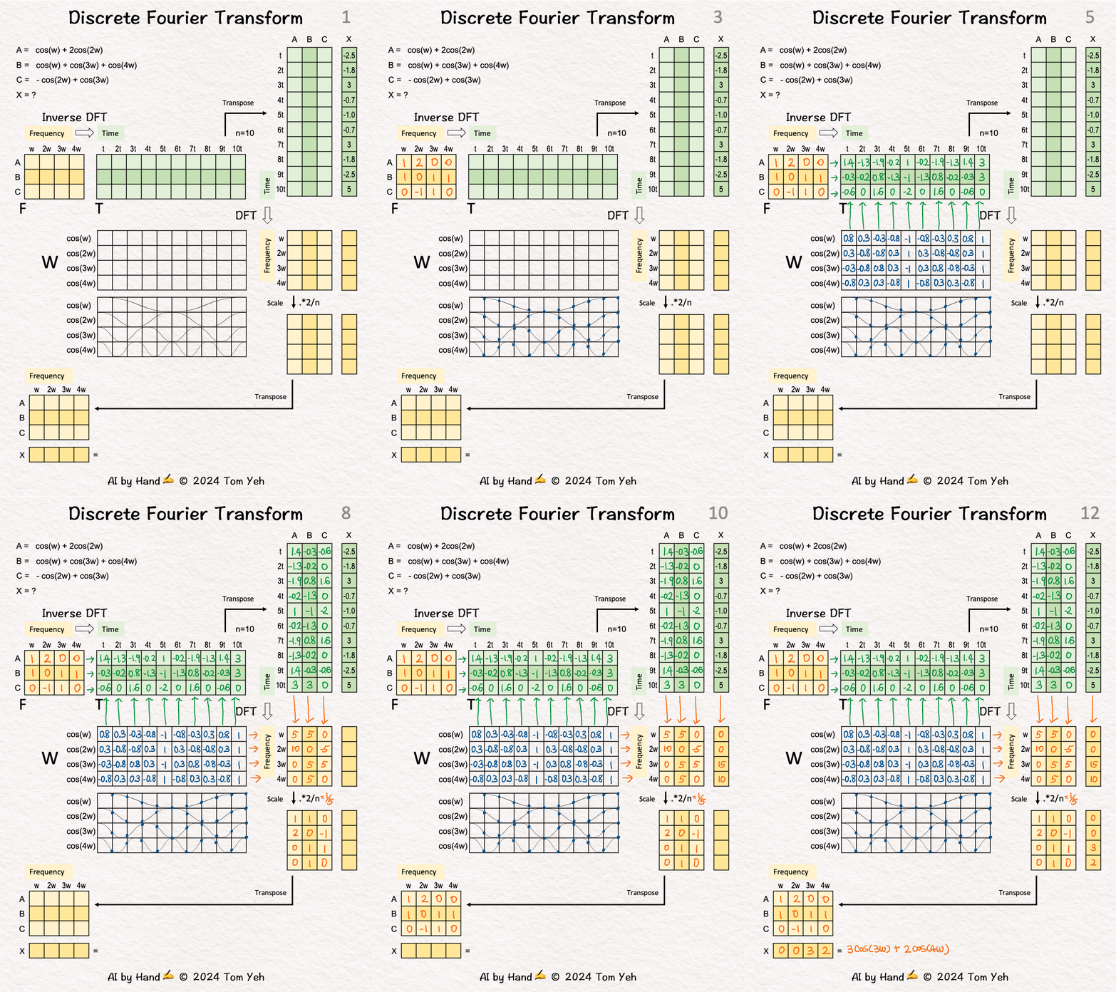
The goal is to take signals from the frequency domain, move them to the time domain via Inverse DFT, and then use the DFT to return them to their original state.
📋 Project Roadmap
- Step 1: Define Frequency Domain Signals
- Step 2: Construct the Frequency Matrix
- Step 3: Discrete Sampling
- Step 4-12: (Remaining calculations)
Step 1 of 12: Frequency Domain Signals
We begin with three signals—A, B, and C—defined in the 🟧 frequency domain. Each is a weighted sum of four cosine waves at frequencies and :
- Signal A:
- Signal B:
- Signal C:
Additionally, we have a signal X sampled at 10 distinct time points ():
X = [-2.5, -1.8, 3, -0.7, -1.0, -0.7, 3, -1.8, -2.5, 5]
Note: X is also a weighted sum of those same four cosine waves, though the weights are currently unknown.
Step 2 of 12: The Frequency Matrix (F)
We can represent the coefficients of signals A, B, and C as a matrix F:
| Signal | ||||
|---|---|---|---|---|
| A | 1 | 2 | 0 | 0 |
| B | 1 | 0 | 1 | 1 |
| C | 0 | -1 | 1 | 0 |
Step 3 of 12: From Continuous to Discrete
The next phase involves taking the continuous cosine waves and extracting discrete samples at the time points through .
🔄 Process Flow
🖼️ Visual Aids




📚 Related "By Hand" Series
- Matrix Multiplication ✍️
- Multi Layer Perceptron (MLP) ✍️
- Backpropagation ✍️
- SVM ✍️
- Batch Normalization ✍️
- Dropout ✍️
- Recurrent Neural Network (RNN) ✍️
- LSTM ✍️
- Deep RNN ✍️
- Self Attention ✍️
- Transformer ✍️
- Autoencoder ✍️
- Variational Auto Encoder (VAE) ✍️
- Sparse Auto Encoder (SAE) ✍️
- Generative Adversarial Network (GAN) ✍️
- Sampling a Sentence ✍️
- Residual Network ✍️
- U-Net ✍️
- Discrete Fourier Transform ✍️
- Graph Convolutional Network (GCN) ✍️
- CLIP ✍️
- Vector Database ✍️
- Mixture of Experts (MoE) ✍️
- Switch Transformer ✍️
- Mamba's S6 ✍️
- Sora's Diffusion Transformer (DiT) ✍️
- BitNet ✍️
- RLHF ✍️