Fractal Jittered Voronoi Partitions
Fractal Jittered Voronoi Partitions
Originally published by BorisTheBrave.Com on 2026-08-29
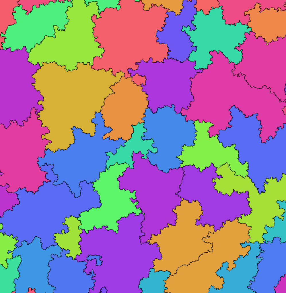
I have discovered a fascinating variation of Voronoi partitions that generates beautiful, fractal-like boundaries for each cell while remaining computationally lightweight.
This technique is particularly well-suited for simulating coastlines, as natural shorelines often exhibit similar fractal characteristics.
Understanding "Jittered" Voronoi
To understand the fractal version, we first need to define Jittered Voronoi. Instead of randomly scattering points across a plane, you begin with an infinite grid of squares. Within every single square, you select one random point—the site.
This is essentially the same logic used in Worley noise, with one key difference: rather than returning the distance to the nearest point, we return the identity of the nearest site, thereby partitioning the plane.
Traditional Voronoi diagrams require complex construction algorithms. In contrast, Jittered Voronoi is highly efficient because it can be computed per-point:
- For any point , identify the surrounding grid cells.
- Determine the site for each of these 25 cells using a hashed pseudo-random number generator (PRNG).
- Identify which of these sites is closest to .
This removes the need to build a global data structure or manage the boundaries of an infinite plane.
The Fractal Procedure
The fractal variant extends this logic through a recursive layering process. Here is the mathematical breakdown:
- Layer 0: Establish an infinite grid and assign a site to each cell via PRNG.
- Layer 1: Create a second grid where the cell size is halved. Assign sites to these smaller cells.
- Parenting: For every site in Layer 1, assign it a "parent" site from Layer 0 (the nearest Layer 0 site).
- Recursion: Repeat this process—halving the grid size and linking sites to the nearest site in the layer immediately above.
The final partition for any given point is determined by tracing the parent chain upward until you reach the root site in Layer 0.
Hierarchy Visualization
Comparison Table
| Feature | Standard Jittered Voronoi | Fractal Jittered Voronoi |
|---|---|---|
| Boundary Shape | Linear/Polygonal | Fractal/Jagged |
| Complexity | Single-layer lookup | Multi-layer recursive lookup |
| Primary Use | Cellular textures | Coastlines, organic borders |
| Computation | local search | local search |
Implementation Details
To handle the infinite nature of the grid and the potential for infinite recursion, we use two strategies:
- Local Search: Only a small, fixed number of cells are relevant for any point at any level.
- Finite Depth: We stop at a specific iteration depth based on the current zoom level, using a standard Voronoi diagram of the final layer as a close approximation.
Core Logic (Python)
from functools import cache
from math import sqrt, floor

# The size of a cell at a given depth: s = 2^(-layer)
def cell_size(layer):
    return 2 ** (-layer)

@cache
def site(layer, cell):
    """Returns the site for grid cell (x, y) using a deterministic hash."""
    s = cell_size(layer)
    offset = hash2(layer, cell) # Returns random pair in [0, 1)
    return s * (cell + offset)

def nearest_site(layer, p):
    """Finds the closest site in layer i to point p."""
    s = cell_size(layer)
    centre_cell = floor(p / s)
    best_distance = float('inf')
    best_site = None

    # A 5x5 search area is mathematically sufficient
    for dx in range(-2, 3):
        for dy in range(-2, 3):
            cell = centre_cell + (dx, dy)
            q = site(layer, cell)
            d = squared_distance(p, q)
            if d < best_distance:
                best_distance, best_site = d, q
    return best_cell, best_site

@cache
def root(layer, cell):
    """Traces a cell's ancestry back to Layer 0."""
    while layer > 0:
        cell = parent(layer, cell)
        layer -= 1
    return cell
Adaptive Stopping Condition
A more optimized approach avoids a fixed depth. If a point is sufficiently close to a site at layer , we can stop early because subsequent layers will not change the root.
The Safety Check:
We define an influence_radius as:
If all potential ancestors within this radius share the same root, the result is "safe."
Adaptive Implementation Checklist
- Calculate
influence_radiusbased on current cell size. - Expand search to a area ( cells) to capture all possible ancestors.
- Collect roots of all sites within the influence radius.
- Break recursion if
len(possible_roots) == 1.
def partition_adaptive(p, max_depth):
    """Computes partition with early exit for efficiency."""
    for layer in range(max_depth + 1):
        cell, _, safe = nearest_site(layer, p, check_safe=True)
        if safe:
            break
    return root(layer, cell)
Visual Result